Project Definition
Project Overview
Path planing has become one of the forefront domains in artificial inteligence. One common application is for the navigation of robots through a maze, such as in Micromouse competitions. To make this possible there are several components. The first, environment sensing, involves the input of data about the environment through physical (or virtual) sensors. The second, SLAM, or simultanious localization and mapping involves the use of this sensor data to create a map of a given area while also maintaining some knowledge of the robot’s position. The final piece is the path planning itself, generally an algorithm using a map of the environment and the location of the goal to plan the next best move.
This project is simulated micromouse competition. A pre-generated maze is provided as well as a few python files to give a framework in which the robot can operate.
maze.py: Loads a maze text file into memory and checks its validity.showmaze.py: Uses turtle to draw a .txt mazetester.py: Tests the robot in a maze
Lasly a template robot inteligence is provided in: robot.py. The majority of the code written for this project is here. It contains an algorithm for mapping, pathing, and drawing the maze from the sensor data.
A much more detailed statement of this project can be found here
Problem Statement
The goal of this project is to implement the create a robot AI that can navigate any maze provided and reach the goal. At each timestep, the robot will recieve sensor data from the tester and return it’s choice of move. To do this the robot will have to do the following:
- Maintain an accurate record of it’s current location
- Create a map of the environment from the sensor data
- Navigate towards the goal
- Do enough exploration to find the optimal path
- Bonus: Create a visualization of the AI (chosen path, explored nodes)
I would expect the robot to be able to navigate any maze given if it has a valid path to the goal as well as to eventually find the optimal path. It should also create a visualization so that one can watch the robot to get an idea of how it is operating.
Metrics
For this project the metric is stated by the competition as a score based on two runs of the maze. The first run is for exploration, while the second run is for reaching the goal as fast as possible.
score = time steps in first run / 30 + time steps in second run
The goal will be to minimize this score.
Analysis
Data Explorations / Visualizations
Up to this point the maze and the robot have been theoretical. Now we will give them substance. The maze will be a grid of n x n squares, where n is an even number. There will be walls along the outside edge of the maze as well as many internal walls through which the robot cannot move. The robot will start on the bottom left corner of the maze and the goal will be any of the four squares in the center of the maze.
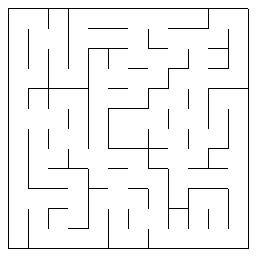
Here is the 12 x 12 maze as an example (from showmaze.py):
As for the robot, it will occupy a single square and point in one of the four cardinal directions. It will also have three sensors on it’s front, left, and right sides. These sensors will give the robot data about the walls. Specifically, each sensor will give an integer value for how many squares away a wall is in the direction of that sensor. In terms of movement, the robot can do two things on it’s turn, move and rotate. It can rotate -90, 0, or 90 degrees clockwise, and it can move forwards or backwards up to three squares.
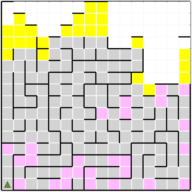
Let’s take a look at that first example maze to get a better idea of what our robot is working with. The first thing that I notice is that the robot will have to move most (or even all) of the way to the right side of the maze to get to the goal. This means that any exploration done on the left half will be fairly useless. The next thing that I noticed is that there seem to be two main paths. One above the goal, and one below. The optimal path will be a variation of one of these. Perhaps the most interesting twist to this problem is that moves of three spaces and moves of one are weighted the same in terms of scoring. This would tend to reward path with fewer turns, rather that simply the shortest distance traveled. With all of this considered, I went to find the optimal path.
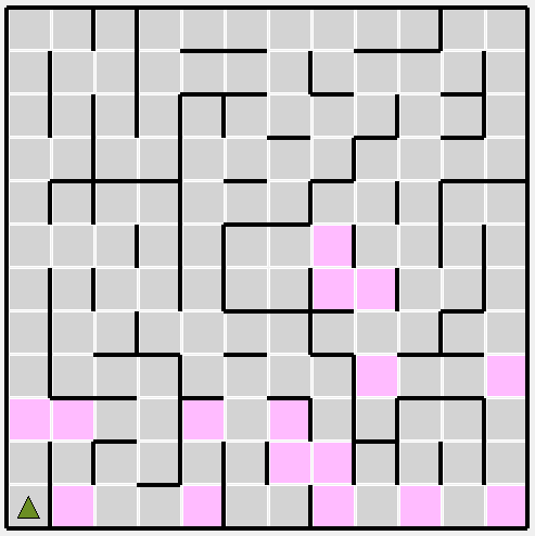
The pink squares are the moves that the robot will make (in this case in the optimal path to the goal). For this maze, the optimal path ended up being 17 moves long.
Benchmark
To determine how efficient the robot is at mapping and path planning for these mazes it would be wise to develop a benchmark, or a score to shoot for. Take the 12x12 maze for example. For this maze the shortest possible path is 17 moves. Therfore, the best possible score would be 17 / 30 (for the first run) + 17 (for the second run), for a best score of 17.6. Since this would be an unrealistic goal (requiring zero wrong moves) we will assume some inefficiency in the exploration phase. If approximately 50% of the cells need to be explored to find the best path this would correlate to 12 x 12 / 2 = 72 cells to explore, which would take 72 moves minimally. The score for this would be 72 / 30 + 17 = 19.4. This process can be similarly performed for each maze size. The results of this are summarized in this table:
| Size | Optimal Path | Goal Score |
|---|---|---|
| 12x12 | 17 | 19.4 |
| 14x14 | 23 | 26.3 |
| 16x16 | 25 | 29.3 |
Methodology
Data Preprocessing
For this project the Data pre-processing was minimal. The only data that the robot recieves is the sensor data. This data is based on heading (forward, left, and right sensors) rather than absolute direction. For my purposes, it was more valuable to have the data in absolute directions, so the sensor data is converted using the heading of the robot to absolute directions (e.g. left, up, down).
Implementation
For this robot to be able to succesfully navigate the maze and find a goal it must perform four main functions:
- Maintain an accurate record of it’s current location
- Create a map of the environment from the sensor data
- Navigate towards the goal
- Do enough exploration to find the optimal path
To perform each of these, a framework needed to be created to hold information about the maze. For this I chose to use a graph, where each node represents one of the cells of the maze. Edges between nodes represent valid, single-move paths between cells.
Maintaing an Accurate Location
This is the simplest of the four by far, but it still has its challenges. The solution used by this robot is to, at each timestep, use the previous sent move to update the current location of the robot. The challenge comes with invalid moves. If the robot were to update it’s position when a move is rejected by the tester as invalid, it would be forever lost. This ends up being a non issue using the graph method to move since we always move along edges (and edges are defined as valid single moves), but with other methods each move would have to be first verified using the sensor data.
Generating a Map
At each time step new information is gained through sensor data. This data is used to add nodes to the graph. For each sensor direction, paths are added for every valid move. For example, if the front sensors sees a wall 5 steps away, lets label the 5 cells in front of the robot c1 through c5. There are 9 valid edges here:
c1 - c2, c1 - c3, c1 - c4
c2 - c3, c2 - c4, c2 - c5
c3 - c4, c3 - c5
c4 - c5
All of these edges would be added to the graph (if they do not already exist). Once this has been done for each of the three sensors, all of the nodes seen by the robot will have been added.
Navigation
To navigate to a given node, a modified version of the breadth-first search algorithm was borrowed from this tutorial by Red Blob Games. Here is the algorithm as implemented in python:
frontier = Queue()
frontier.put(self)
came_from = {}
came_from[self] = None

while not frontier.empty():
    current = frontier.get()
    for node in current.edges:
        if node not in came_from:
            frontier.put(node)
            came_from[node] = current

current = other
path = []
while current != self:
    path.append(current)
    current = came_from[current]
path.reverse()
return path
self refers to the node currently occupied by the robot.
other refers to the node we are navigating to
Since breadth-first search always finds the optimal path this algorithm guarantees that we take the best path between two nodes.
Exploration
The breadth-first algorithm described in the previous section is good but it cannot explore new nodes, only plan a path to nodes have already been seen. To remedy this we need another path planning algorithm one level above this. This algorithm works as follows:
- Each time a new node is added to the graph it is also added to a frontier set
- When a node is visited it is removed from the frontier
- If there is not currently a path being followed, choose a new frontier node to move to
- Find the path to this node using the breadth-first algorithm above
- Move along this path
How this path is chosen is borrowed from heuristic search algorithms like A*. Each node on the frontier is scored based on a combination of aspects. The wrinkle for this specific problem is that this combination changes depending on the phase of exploration that the robot is in. There are two runs of the maze. At the start of the second run we will have already found a path to the goal and attempted to refine it. For this reason, no heuristic is needed. Simply navigate to the goal with breadth first search. However, durring the first run, the robot must both find the goal, and explore for the optimal path. Because of this, the first run can be split up into two phases: The first pahse is for simply finding the goal. In the second phase, once the goal has been found, the goal is to explore some portion of the rest of the maze to find the optimal path from start to goal.
For each of these phases, nodes on the frontier are scored as follows:
score = (
    self.weight1_goal_dist * node.distance(self.goal_node)
    + self.weight1_self_dist * node.distance(self.cur_node)
    + self.weight1_area_explored * self.area_explored(node)
)
weight1 corresponds to the weight during phase one (find goal), while weight2 would be for phase two (exploration). The first run is ended when a percentage of cells in the maze have been explored. This is defined by the explore_percent of the robot. The six weights for the heuristic and this explore_percent are the hyper-parameters of the robot. These parameters could be tuned to optimize the performance of the robot.
Refinement
Towards the beginning of this project I was not using two separate round one phases, or even the distance to the current node as part of the heuristic. This resulted in a robot acting similar to a greedy search algorithm. By greedy I mean that it was always trying to explore the node closest to the goal. It would make very long movements up and down the height of the maze just to make one cell of progress at each of the disparate paths. It also would not find the optimal path, since it would begin run two as soon as it found the goal. A typical score for these runs was 28.7 on the 12x12 test maze. The next step was to add distance from the current node to the heuristic. Interestingly, this created closer of a depth first greedy algorithm, as the robot was likely to explore it’s current path. After some tuning of the weights, (1 for the distance to the goal, 2 for the distance from the current node) this algorithm managed a score of 23.9 on the 12x12 maze. The last step was to add the second phase. For this phase the goal is to find the optimal path by exploring more of the maze. After tuning these parameters (0 for the goal distance weight, 1 for the self distance weight, 0.7 for the explore percent), this algorithm managed a score of 22.0 on the 12x12. The last improvement I attempted was to add an area explored measure to the heuristic. This was defined as follows:
# Max score ~maze_dim for corner node with nothing visited
score = 0
for n in self.maze_map:
    if n == node:
        continue
    if n not in self.visited:
        dist = node.distance(n)
        score += 1 / dist

return score
From some manual attempts to tune the weights on this score I was not able to find a combination of parameters that gave a better score. Because of this the weights for this heuristic were left at 0.
The next task was to attempt to tune the hyper-parameters. For this task I used a brute force method. The robot was run a few thousand times through each maze. Each time with a set of random hyper-parameters with the following ranges (inclusive on both ends):
| Parameter | Low | High | Interval |
|---|---|---|---|
| explore_percent | 0 | 1 | 0.1 |
| weight1_goal_dist | 0 | 4 | 1 |
| weight1_self_dist | 0 | 4 | 1 |
| weight1_area_explored | 0 | 4 | 1 |
| weight2_goal_dist | 0 | 4 | 1 |
| weight2_self_dist | 0 | 4 | 1 |
| weight2_area_explored | 0 | 4 | 1 |
The result of each run was written as an entry in a csv along with the maze dimentions and the parameters used. By grouping these entries by the parameters used and sorting by the sum of scores across the three mazes I was able to find a combination of parameters that were effective for all of the mazes in question. The weights for explored area for each run are ommitted since the best value was zero for all of the best scores.
| explore_percent | w1_goal | w1_self | w2_goal | w2_self | sum score |
|---|---|---|---|---|---|
| 0.5 | 1 | 3 | 2 | 3 | 82.46 |
Results
Model Evaluation and Validation
Using this random scattershot approach I was able to find sets of parameters that performed very well for each of the three starter mazes. For each of these tables the parameters will be listed as one value with the format of explore_percent: weight1_goal_dist - weight1_self_dist - weight2_goal_dist - weight2_self_dist. The area explored weights will be omitted as they were 0.
| Size | Optimal Path | Goal Score | My Score | Parameters |
|---|---|---|---|---|
| 12x12 | 17 | 19.4 | 20.3 | 0.1: 1-3-0-3 |
| 14x14 | 23 | 26.3 | 29.0 | 0.5: 1-2-3-3 |
| 16x16 | 25 | 29.3 | 31.1 | 0.0: 1-3-2-3 |
Notice the explore_percent of close to zero for the 12x12 and 16x16 mazes. In each of these cases, the optimum path is found during the find goal phase of the first run. This is essentially an overfitting of the parameters to those specific mazes. To attempt to remedy this the parameters found in the previous section that take into account the sum of scores accross all three mazes will be used. Here are those parameters:
| explore_percent | w1_goal | w1_self | w2_goal | w2_self |
|---|---|---|---|---|
| 0.5 | 1 | 3 | 2 | 3 |
For this set of parameters, these were the scores on each of the three test mazes:
| Size | Optimal Path | Goal Score | My Score |
|---|---|---|---|
| 12x12 | 17 | 19.4 | 21.0 |
| 14x14 | 23 | 26.3 | 28.0 |
| 16x16 | 25 | 29.3 | 32.4 |
Conclusion
Reflection
This project consisted of desinging a simple robot AI to navigate a maze. This robot had to perform 5 main functions to succed at this task:
- Maintain an accurate record of it’s current location
- Create a map of the environment from the given sensor data
- Navigate towards the goal
- Exploration enough to find the optimal path
It was scored based on a combination of the time it spent exploring and the time for the best path. To inplement this AI, I Gathered sensor data into a graph structure containing nodes for each square in the maze and edges between them. Then I used a heuristic based search to determine the next square to navigate towards. Finally, I tuned the weights in this heuristic search until an acceptable score was achieved.
This project was especially difficult because the search was performed online and without full information of the maze. This differs from typical search in that after each move the knowledge that the robot possesses must be re-evaluated, which adds a significant wrinkle to the typical search methods. On the other hand, this is also a much more practical situation for path planning, which made the project much more interesting as well.
Improvement
The unfortunate truth of this path planning algorithm is that a lot of information is not fully used. For instance, cells that have been passed over in a move of more than one square should probably be weighted less on the frontier. Additionally, sections of the maze could probably be ruled as not needed to be explored with sufficient knowedge of their surroundings. These types of things would be taken into account by algorithms that confirm optimality of the path. The challenge is performing these algorithms online.
Another area of improvement would be to make the AI more robust against larger mazes. This algorithm is not optimized for speed, but for simplicity (and reliability). For this reason, and since the search space grows with n^2 (where n is the size of the maze), this algorithm would not scale well.
Finaly, in future iterations of the project, I would like to continue to tune the hyper-parameters in a more organized manner (rather than brute force). To do this more mazes would be needed as well as a better way than randomized values for chosing parameters programatically. This would allow for a more robust search of the solution space and hopefully yeild better results.